Beyond the MLP
All slides — click to jump · Esc to close

Keyboard shortcuts

→ Space PgDnnext step / slide
← PgUpprevious
O · Escslide overview
Ashow / hide step-by-step reveals
Tpresenter timer (R resets it)
Ffull screen
Home Endfirst / last slide

Each slide has its own address (e.g. #convlab). Arrow keys stop working while the cursor is inside an embedded tool — click outside it or use the ‹ › buttons.

Introduction to Machine Learning and Data Mining 2026/27 · Class 8: Deep Learning

Beyond the MLP: from convolutions to generating images

Convolutional networks, autoencoders and GANs — and an intuition for recurrent networks, transformers and ChatGPT.

Use → / ← or the arrow buttons · ? for shortcuts

Storyline

Every architecture is a bet about the structure of the data

1

MLP

A flat vector of features. Assumes no structure. Learns its own features.

2

CNN

Space: patterns are local and repeat. Locality + weight sharing.

3

Autoencoder

Learns a compact code by rebuilding its input — no labels.

4

GAN

Generates new data through an adversarial game.

5

RNN · LSTM

Time: reads in order and carries a memory. Intuition only.

6

Transformer

Attention: every word can look at every other. Intuition only.

7

ChatGPT

Next-word prediction at scale, tuned with human feedback. Intuition only.

The thread

Throughout, networks learn representations of the data with the same training loop (loss → backpropagation → update). What changes is which connections exist — the assumption about the data's structure.

SourcesGoodfellow, Bengio & Courville (2016); Bengio, Courville & Vincent (2013) — full references at the end.
Act 1 · The MLP and why depth · recap

An MLP is a stack of “linear map + non-linearity” layers, trained by gradient descent

Dense layer

Every unit sees every input. Parameters = inputs × units + units.

Learning

Forward pass → loss → backpropagation → update (Rumelhart et al., 1986).

Expressive in principle

One hidden layer can approximate any continuous function (Cybenko, 1989; Hornik et al., 1989) — but that says nothing about how many units are needed, or how learnable it is.

SourcesRumelhart, Hinton & Williams (1986); Cybenko (1989); Hornik, Stinchcombe & White (1989); Goodfellow et al. (2016) ch. 6; course Class 5 (slides 6–20).
Act 1 · Why deep learning

A hidden layer re-represents the data so that a simple classifier suffices

Raw inputs: no line works

XOR: a linear model scores ≈ 50 % — the classic limitation of the single-layer perceptron (Minsky & Papert, 1969).

Learned features: a line works

The hidden layer learns new coordinates (h₁, h₂) in which the classes are linearly separable — features and classifier are learned together.

“Representation learning”

The main advantage of neural networks over manual feature engineering (Bengio et al., 2013). Deeper nets repeat the step.

SourcesGoodfellow et al. (2016) §6.1 (learning XOR); Minsky & Papert (1969); Bengio, Courville & Vincent (2013); Olah (2014), Neural networks, manifolds and topology; course Class 5 (slides 6, 39–41). Live demo: 240 points, trained in your browser.
Act 1 · Why deep learning

Stacking layers builds a hierarchy: simple features are composed into abstract ones

Empirical evidence

In trained image CNNs, early layers respond to edges and colour, middle layers to textures and parts, late layers to object-level patterns (Zeiler & Fergus, 2014; Olah et al., 2017).

Biological inspiration

Hierarchical visual processing (Hubel & Wiesel, 1962) inspired the Neocognitron (Fukushima, 1980) and, through it, CNNs.

Same logic in language

Characters → words → phrases → meaning: see the “Text” tab.

SourcesZeiler & Fergus (2014); Olah, Mordvintsev & Schubert (2017); Goodfellow et al. (2016) Fig. 1.2; Hubel & Wiesel (1962); Fukushima (1980). The drawings are schematic, after Goodfellow et al. (2016) Fig. 1.2 — not outputs of a trained model.
Act 2 · CNNs · handling images

To a network, an image is a grid of numbers — one grid per colour channel

Height × width × channels

A greyscale image has 1 channel (brightness); a colour image has 3 (red, green, blue), each a number from 0 to 255.

Neighbours are related

Look at the highlighted 3×3 patch: in smooth regions the numbers barely change; at an edge they jump. Patterns live in local neighbourhoods.

And there are a lot of them

Even a small photo has hundreds of thousands of numbers — the problem the next slides address.

SourcesGoodfellow et al. (2016) ch. 9 (introduction); Zhang et al., Dive into Deep Learning §7.1. The colour picture is a toy drawn for this slide; the digit is from the UCI Optical Recognition of Handwritten Digits data (Alpaydin & Kaynak).
Act 2 · The case for CNNs (1/3) · size

Images are too big for dense layers: the parameter count explodes

≈ 150 million weights

One dense layer of 1,000 units on a 224 × 224 colour photo (150,528 inputs) — about 600 MB, before adding a second layer.

Overfitting risk

Far more parameters than examples: the network can memorise instead of generalise.

A convolutional layer does not grow with the image

64 filters of 3 × 3 × 3 = 1,792 parameters, whatever the image size.

SourcesGoodfellow et al. (2016) §9.2; Zhang et al., Dive into Deep Learning §7.1; course Class 5 (slides 9–11: counting dense-layer parameters) and the MNIST exercise (795,010 parameters).
Act 2 · The case for CNNs (2/3) · structure

Flattening discards what makes an image an image: its spatial structure

The MLP receives a list, not a picture

Pixel 17 and pixel 18 are just two inputs; the pixel below pixel 17 is number 25. Neighbourhood is not represented anywhere.

The proof: permute the pixels

Shuffle every image with the same random permutation and an MLP learns equally well (the “permutation-invariant MNIST” setting). A human — or a CNN — could not.

What we know and the MLP does not

① Nearby pixels form meaningful patterns. ② A pattern means the same wherever it appears. → Build both into the architecture.

SourcesGoodfellow et al. (2013), Maxout networks (permutation-invariant MNIST); Goodfellow et al. (2016) §9.2; LeCun et al. (1998). Digits: UCI Optical Recognition of Handwritten Digits (Alpaydin & Kaynak).
Act 2 · The case for CNNs (3/3) · the two priors

The fix: build in locality and weight sharing

Locality (sparse connectivity)

Each unit looks at a small neighbourhood. Far fewer connections; units detect local patterns.

Weight sharing

The same filter is applied at every position: far fewer parameters, and a pattern is found wherever it occurs (translation equivariance).

Where the idea comes from

Local receptive fields (Hubel & Wiesel, 1962) → Neocognitron (Fukushima, 1980) → backpropagation on zip codes (LeCun et al., 1989) → LeNet-5 (LeCun et al., 1998).

These are assumptions

Right for images, audio, time series. Wrong for a spreadsheet: neighbouring columns “age, income, region” mean nothing.

SourcesGoodfellow et al. (2016) §9.2 (sparse interactions, parameter sharing, equivariance); Hubel & Wiesel (1962); Fukushima (1980); LeCun et al. (1989, 1998).
Act 2 · How CNNs work (1/6) · the layer types

A CNN is built from three types of layers

Feature extractor

Convolution (+ ReLU) and pooling layers turn the image into feature maps, from local patterns to larger ones.

Classifier

Flatten + dense layers (+ softmax) turn the features into class probabilities: the MLP from Class 5.

What is learned

Only convolutional and dense layers have parameters; pooling has none. All are trained together by backpropagation.

SourcesLeCun, Bottou, Bengio & Haffner (1998); Goodfellow et al. (2016) §9.1–9.3; Zhang et al., Dive into Deep Learning ch. 7.
Act 2 · How CNNs work (2/6) · the convolutional layer

A filter is a small pattern detector slid across the image; its output is a feature map

Operation

Slide a k×k kernel; at each position multiply the patch by the kernel and add up. out(r,c) = Σᵢⱼ patch(r+i, c+j) · kernel(i,j)

Feature map

Shows where the pattern occurs: orange = match, blue = opposite pattern. ReLU keeps only positive evidence.

Max-pooling

The pooling layer keeps the strongest response in each block: half the size, a little tolerance to shifts.

SourcesGoodfellow et al. (2016) §9.1, §9.3; Zhang et al., Dive into Deep Learning §7.2; Powell, Image kernels explained visually (setosa.io). Strictly this is cross-correlation (no kernel flip), which is what deep-learning libraries call “convolution”.
Act 2 · How CNNs work (3/6) · a convolutional layer in detail

A layer applies many filters at once — and the filters are learned, not designed

InputH × W × Cine.g. 224×224×3 F filterseach k × k × Cine.g. 64 × (3×3×3) slidestack Feature mapsH′ × W′ × Fe.g. 222×222×64
Each filter spans all input channels

A filter on an RGB image is 3×3×3 = 27 weights + 1 bias. A layer with F filters gives F feature maps.

parameters = F · (k·k·Cin + 1)
output size = ⌊(n + 2p − k) / s⌋ + 1
The numbers in the filters are learned

Random start, then the same training loop as the MLP. In trained image networks the first-layer filters typically look like edge and colour detectors (Krizhevsky et al., 2012, Fig. 3).

Worked example

64 filters of 3×3 on an RGB photo: 64 × (27 + 1) = 1,792 parameters. (n = input size, k = kernel size, p = padding, s = stride.)

SourcesKrizhevsky, Sutskever & Hinton (2012) Fig. 3; Zhang et al., Dive into Deep Learning §7.3–7.4 (padding, stride, channels); Goodfellow et al. (2016) ch. 9. The size formula holds when stride and padding divide evenly.
Act 2 · How CNNs work (4/6) · depth

Stacking layers — and pooling — grows what each unit can see: that is the hierarchy

Convolutions add slowly

Every filter is tiny, but each 3×3 conv adds only 2 pixels to the receptive field (the region a unit depends on): 3 → 5 → 7 …

Pooling accelerates it

Downsampling makes later filters cover more of the original image: conv → pool → conv → pool reaches 3 → 4 → 8 → 10.

Link to the hierarchy

Small receptive field → edges; large → parts and objects. In practice the effective receptive field is smaller than the theoretical one (Luo et al., 2016).

SourcesGoodfellow et al. (2016) §9.2; Luo, Li, Urtasun & Zemel (2016); Zeiler & Fergus (2014). Shown here: valid 3×3 convolutions, stride 1, and 2×2 pooling with stride 2.
Act 2 · How CNNs work (5/6) · putting it together (28×28 digits)

A CNN classifier = a learned feature extractor + the MLP you already know

5,258 parameters in total

80 + 1,168 + 4,010 — versus 795,010 for the dense 784 → 1000 → 10 network from the course exercise.

Convolution and pooling extract; dense layers decide

The last blocks are the Class 5 classifier: softmax over classes, cross-entropy loss.

Lineage

LeNet-5 (LeCun et al., 1998) in spirit: convolution → pooling → … → fully connected, trained end-to-end by backpropagation.

SourcesLeCun, Bottou, Bengio & Haffner (1998); Zhang et al., Dive into Deep Learning §7.6 (LeNet); course Class 5 (slides 35–38: softmax, cross-entropy).
Act 2 · How CNNs work (6/6) · why it mattered

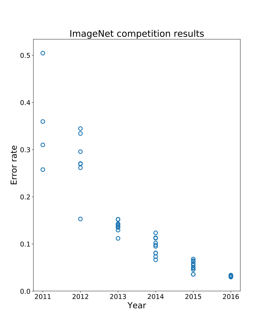
Deep CNNs reset computer vision in 2012

Scatter plot of the best ImageNet competition result of each team per year, with error rate on the vertical axis. In 2012 one entry, AlexNet, lies far below all the others, and error keeps falling in the following years.
Real results of the ImageNet classification competition (best entry per team, up to 10 entries per year). Figure: Gkrusze (2018), “ImageNet error rate history (just systems)”, Wikimedia Commons, CC BY-SA 4.0 (source). Data: ILSVRC results (Russakovsky et al., 2015).
The 2012 jump

The lone point far below all others is AlexNet (≈ 60 M parameters, trained on two GPUs): 15.3 % top-5 error vs. 26.2 % for the runner-up (Krizhevsky et al., 2012).

Then: deeper

8 → 22 → 152 layers; by 2015 residual networks reached 3.6 % (He et al., 2016) — below the 5.1 % of one trained human annotator on this benchmark (Russakovsky et al., 2015).

Why it matters for social science

Satellite imagery to estimate poverty (Jean et al., 2016); audits showing face-analysis systems err far more on darker-skinned women (Buolamwini & Gebru, 2018).

SourcesRussakovsky et al. (2015); Krizhevsky et al. (2012); He et al. (2016); Jean et al. (2016); Buolamwini & Gebru (2018). The figure is reproduced unmodified from Wikimedia Commons under its licence.
Act 2 · Live demo · a trained CNN, layer by layer

All the pieces in one trained network

Loading CNN Explainer…
The same layers

Input 64×64×3 → conv → conv → pool → conv → conv → pool → softmax over 10 classes (“Tiny VGG”).

Filters and maps

Click a conv_1_1 neuron: 3 kernels (one per colour channel) of 3×3; the layer has 10 × 3 × 9 + 10 = 280 parameters.

Depth

Early maps are fine; late maps are coarser and more class-specific — the hierarchy.

Use ⤢ Full width (top right) — the tool needs room.

SourceWang, Turko, Shaikh, Park, Das, Hohman, Kahng & Chau (2021), CNN Explainer, IEEE TVCG. poloclub.github.io/cnn-explainer (embedded, © the authors).
Act 3 · Autoencoders · learning without labels

An autoencoder compresses an input into a code and rebuilds it — the input is its own label

xinput64 pixels Encodercompress z BOTTLENECKk numbers(the “code”) Decoderrebuild x̂output64 pixels loss: how different is x̂ from x? L = ‖x − x̂‖²
Classifier (CNN)
x → features → label (needs labels)
Autoencoder
x → code → x̂ ≈ x (the input is the label)
Encoder: x → z

Compresses the input into a code with far fewer numbers (the bottleneck). For images it can be the convolutional stack we just built.

Decoder: z → x̂

Rebuilds the input from the code alone (convolutional decoders use up-sampling or transposed convolutions).

Learning

Minimise the reconstruction error with the same backprop. No labels: unsupervised / self-supervised.

Relation to PCA

With linear layers and squared error the code spans PCA’s subspace (Baldi & Hornik, 1989); non-linear layers go beyond it (Hinton & Salakhutdinov, 2006).

SourcesHinton & Salakhutdinov (2006); Baldi & Hornik (1989); Goodfellow et al. (2016) ch. 14; Weng (2018), From autoencoder to Beta-VAE.
Act 3 · Live: a real autoencoder, trained in your browser

Two numbers can rebuild a digit — and the code organises itself without labels

Signal = reconstruction

Trained on unlabeled digits; the error falls from the “average digit” baseline.

Structure emerges

Digits cluster in the code space although labels were never used (colours show the true digit, for display only).

Holes

Between clusters the decoder produces blobs: rebuilding ≠ generating.

MethodOwn implementation: 64 → 32 → k → 32 → 64, tanh hidden units, sigmoid output, Adam, minibatch 32. Data: 1,000 images from the UCI Optical Recognition of Handwritten Digits set (Alpaydin & Kaynak), 8×8 pixels; 800 for training, 200 held out. For k > 2 the map shows a 2-D (PCA) projection of the code.
Act 3 · What makes a learned code useful

A good code is compact, informative, organised and reusable — the bottleneck is the design knob

Compact

Far fewer numbers than the input (64 → 2…16).

Informative

The input can be (largely) rebuilt from it.

Organised

Similar inputs lie close together in code space.

Reusable

Feeds clustering, search, classification with few labels, anomaly detection.

The bottleneck trade-off

Too wide: the network can copy its input (the identity) and learn nothing. Too narrow: blurry rebuilds. Zero error is not the goal. A common cure for the identity shortcut: denoising autoencoders, which rebuild the clean input from a corrupted one (Vincent et al., 2008).

SourcesGoodfellow et al. (2016) §14.1–14.5; Vincent, Larochelle, Bengio & Manzagol (2008); Bengio, Courville & Vincent (2013).
Act 3 · Learned codes in practice · embeddings

Learned codes are called embeddings — and they are used everywhere

manwomankingqueen “female”“royal” king − man + woman ≈ queen
Schematic of the idea in 2-D — not real coordinates. Real embeddings have 100s of dimensions (Mikolov et al., 2013).
Words → meaning as geometry

word2vec places words with similar meanings close together; directions encode relations such as gender or royalty (Mikolov et al., 2013).

Social science with word embeddings

Embeddings trained on 100 years of text quantify changing gender and ethnic stereotypes (Garg et al., 2018); map the meaning of “class” (Kozlowski et al., 2019); place parties and politicians on ideological scales from speeches (Rheault & Cochrane, 2020).

Faces and images

FaceNet maps each face to a 128-number embedding: photos of the same person land close together, different people far apart — used for verification and clustering (Schroff et al., 2015).

Recommendations

YouTube represents videos and users as embeddings and retrieves candidates by proximity (Covington et al., 2016).

Networks

node2vec embeds each node of a network, e.g. for link prediction and community detection (Grover & Leskovec, 2016).

SourcesMikolov et al. (2013a, 2013b); Garg, Schiebinger, Jurafsky & Zou (2018); Kozlowski, Taddy & Evans (2019); Rheault & Cochrane (2020); Schroff, Kalenichenko & Philbin (2015); Covington, Adams & Sargin (2016); Grover & Leskovec (2016).
Break

Break — 10 minutes

Second half: GANs, then an intuition for recurrent networks, transformers and ChatGPT.

Act 4 · GANs · from rebuilding to creating

To create, a model must capture how the data is distributed — not just where the boundary is

TaskQuestionModelsExamples
Discriminate“Which class is this x?”p(y | x)CNN classifier, logistic regression
Reconstruct“Can you rebuild this x from its code?”x → z → x̂Autoencoder
Generate“Make a new x that looks like the data.”x ~ p(x)VAE, GAN, diffusion, language models
SourcesNg & Jordan (2001); Goodfellow et al. (2016) ch. 20; Kingma & Welling (2014) (VAEs shape the latent space so it can be sampled). Toy data: two Gaussian classes; the classifier is the exact Bayes posterior for those Gaussians.
Act 4 · GANs · adversarial training

GANs turn generation into a game: a forger (generator) against a detective (discriminator)

Real dataphotos from the dataset noise zrandom numbers Generator Gthe forger fake sampleG(z) Discriminator Dthe detective P(real)0 = fake … 1 = real feedback: “here is how to fool me” update D → better detective update G → better forger
minG maxD V(D,G) = Ex∼p_data[log D(x)] + Ez∼p_z[log(1 − D(G(z)))]
  1. Forge. G turns random noise into a fake sample.
  2. Judge. D sees real and fake samples and outputs P(real); it is trained to classify correctly.
  3. Improve the forger. G is trained so that D calls its fakes “real”; the gradient flows through D into G. G never sees real data directly.
  4. Repeat. Both improve in turn. At the theoretical optimum G matches the data and D can only guess: D(x) = ½ (Goodfellow et al., 2014).
Link to what we built

G has the shape of a decoder (noise instead of a code → image) and D is a classifier. In DCGAN both are CNNs: D a convolutional classifier, G built from transposed convolutions (Radford et al., 2016).

SourcesGoodfellow et al. (2014); Goodfellow (2016), NIPS tutorial: GANs; Radford, Metz & Chintala (2016).
Act 4 · GANs · live demo: adversarial training in action

The discriminator’s verdict reshapes the generator’s samples, step by step

Loading GAN Lab…
Setting

2-D toy data. Green dots = real samples, purple dots = G’s fakes.

D’s opinion

Background colour = D’s P(real): green “looks real”, purple “looks fake”.

G’s learning signal

Pink lines = the gradient through D telling each fake where to move.

Over time

Fakes migrate onto the real data and D’s map flattens.

To start from scratch: untick “Use pre-trained model”, press ↺, then ▶. Use ⤢ Full width (top right).

SourceKahng, Thorat, Chau, Viégas & Wattenberg (2019), GAN Lab, IEEE TVCG. poloclub.github.io/ganlab (embedded, © the authors).
Act 4 · GANs · how good can they get?

Which face is real?

Loading Which Face Is Real?…
One of each pair is generated

Every pair has one real photograph and one face generated by StyleGAN (Karras et al., 2019).

Five years apart

The first GAN samples (2014) were small and blurry (Goodfellow et al., 2014); StyleGAN faces are hard to tell from photographs.

If the page looks cramped, use ⤢ Full width or open it in its own tab.

SourceBergstrom & West, Which Face Is Real?, University of Washington (Calling Bullshit project), whichfaceisreal.com (embedded, © the authors); Karras, Laine & Aila (2019); Goodfellow et al. (2014).
Act 5 · Beyond images · sequences (intuition)

In language, order carries meaning — a bag of numbers cannot see it

Order and variable length

“Dog bites man” ≠ “man bites dog”, and sentences have no fixed length — both trouble an MLP.

Long-range context

“The keys to the cabinet in the hall are missing”: the verb depends on a word far away, beyond a conv window.

SourcesElman (1990); Goodfellow et al. (2016) ch. 10 (introduction).
Act 5 · Beyond images · recurrent networks (intuition)

An RNN reads one word at a time, carrying a memory

The same cell at every step

One set of weights is reused at every step — the trick of a conv filter, but over time instead of space.

The memory is a fixed-size summary

Everything read so far is squeezed into one vector, so long-ago information fades.

LSTM: a protected memory

LSTMs add learned gates that decide what to keep, forget and output, so important information survives longer (Hochreiter & Schmidhuber, 1997).

SourcesElman (1990), Finding structure in time; Hochreiter & Schmidhuber (1997); Goodfellow et al. (2016) §10.1–10.2, §10.10.
Act 5 · Beyond images · transformers (intuition)

Attention lets every word look at every other word directly

Three ways to connect words

A CNN’s view grows slowly with depth; an RNN passes information along a chain; attention connects any two words in one step.

Where it came from

Attention was first added to RNN translation models (Bahdanau et al., 2015); transformers (Vaswani et al., 2017) built whole networks from it.

SourcesVaswani et al. (2017) §4 (why self-attention); Bahdanau, Cho & Bengio (2015).
Act 5 · Beyond images · transformers (intuition)

Self-attention: each word decides which other words matter, and blends them in

Ask, match, blend

Each word has a query (what I look for), a key (what I offer for matching) and a value (what I contribute). Better matches get more attention; the word becomes a blend of the others.

A transformer stacks this

Many attention layers (each followed by an MLP), with word positions added so order is not lost — otherwise it would see a bag of words, like the shuffled pixels (Vaswani et al., 2017).

SourcesVaswani et al. (2017) §3; Alammar (2018), The Illustrated Transformer (the “animal … it” example). The numbers above are a hand-made 2-D toy to show the mechanism — not output of a trained model.
Act 5 · Beyond images · ChatGPT (intuition)

ChatGPT is a transformer trained to predict the next word — then tuned to be helpful

1 · PRE-TRAINING

Predict the next word

On huge amounts of text; the text provides its own labels.

›
2 · INSTRUCTION TUNING

Learn from examples

Humans write good answers to instructions.

›
3 · HUMAN FEEDBACK

Learn from preferences

Humans rank answers; the model is steered towards the preferred ones.

›
RESULT

ChatGPT

Released November 2022 (OpenAI, 2022).

Generation = predict, pick, repeat

The model gives a probability for every possible next word; one is picked (the temperature controls how adventurous), appended, and the loop repeats.

Fluent is not the same as true

It produces plausible text learned from its training data, including that data’s gaps and biases (Ouyang et al., 2022; Bender et al., 2021).

SourcesRadford et al. (2018); Ouyang et al. (2022); OpenAI (2022), Introducing ChatGPT; Bender, Gebru, McMillan-Major & Shmitchell (2021). The demo is a word-pair table counted from a 111-word text written for this class; it illustrates the loop, not ChatGPT’s quality.
Synthesis

Each architecture is a bet on the structure of the data

ArchitectureAssumes about the dataKey mechanismGood forMain limitation
MLPno structure (a flat vector)dense layers, backproptabular dataimages and text are large and structured
CNNlocal, repeated patterns on a gridfilters, weight sharing, poolingimages, audioneeds labels; fixed local view
Autoencoderdata lies near a low-dimensional structurebottleneck, reconstructioncompact codes, embeddings, anomaliescodes are not guaranteed samplable
GANa critic can judge realismgenerator vs. discriminatorsharp synthetic imageshard to train; mode collapse
RNN · LSTMorder mattersmemory, gatessequencesslow; memory fades
Transformerany word may relate to any otherattentionlanguage, and moredata- and compute-hungry
ChatGPTlanguage is predictablenext-word prediction + human feedbackassistantsfluent but not always true
Take-away

The shared thread is representations. Match the architecture to the structure of your data — and audit what the training data bakes in.

SourcesSynthesis of the preceding slides; see the reference list. On inductive bias: Goodfellow et al. (2016) ch. 9.
References (1/2)

From the MLP to autoencoders and embeddings

MLPs and representations

Bengio, Y., Courville, A., & Vincent, P. (2013). Representation learning: A review and new perspectives. IEEE TPAMI, 35(8), 1798–1828.

Cybenko, G. (1989). Approximation by superpositions of a sigmoidal function. Mathematics of Control, Signals and Systems, 2, 303–314.

Goodfellow, I., Bengio, Y., & Courville, A. (2016). Deep Learning. MIT Press. deeplearningbook.org

Hornik, K., Stinchcombe, M., & White, H. (1989). Multilayer feedforward networks are universal approximators. Neural Networks, 2(5), 359–366.

Minsky, M., & Papert, S. (1969). Perceptrons. MIT Press.

Nielsen, M. A. (2015). Neural Networks and Deep Learning. Determination Press. neuralnetworksanddeeplearning.com

Olah, C. (2014). Neural networks, manifolds, and topology. colah.github.io.

Rumelhart, D. E., Hinton, G. E., & Williams, R. J. (1986). Learning representations by back-propagating errors. Nature, 323, 533–536.

Hierarchy, locality, CNNs

Fukushima, K. (1980). Neocognitron. Biological Cybernetics, 36, 193–202.

Goodfellow, I., Warde-Farley, D., Mirza, M., Courville, A., & Bengio, Y. (2013). Maxout networks. ICML.

Hubel, D. H., & Wiesel, T. N. (1962). Receptive fields, binocular interaction and functional architecture in the cat’s visual cortex. J. Physiology, 160, 106–154.

LeCun, Y., et al. (1989). Backpropagation applied to handwritten zip code recognition. Neural Computation, 1(4), 541–551.

LeCun, Y., Bottou, L., Bengio, Y., & Haffner, P. (1998). Gradient-based learning applied to document recognition. Proc. IEEE, 86(11), 2278–2324.

Krizhevsky, A., Sutskever, I., & Hinton, G. E. (2012). ImageNet classification with deep convolutional neural networks. NeurIPS, 25.

Luo, W., Li, Y., Urtasun, R., & Zemel, R. (2016). Understanding the effective receptive field in deep convolutional neural networks. NeurIPS, 29.

Olah, C., Mordvintsev, A., & Schubert, L. (2017). Feature visualization. Distill.

Zeiler, M. D., & Fergus, R. (2014). Visualizing and understanding convolutional networks. ECCV.

ImageNet and applications

Gkrusze (2018). ImageNet error rate history (just systems). Wikimedia Commons, CC BY-SA 4.0.

Russakovsky, O., et al. (2015). ImageNet Large Scale Visual Recognition Challenge. IJCV, 115, 211–252.

He, K., Zhang, X., Ren, S., & Sun, J. (2016). Deep residual learning for image recognition. CVPR.

Jean, N., et al. (2016). Combining satellite imagery and machine learning to predict poverty. Science, 353(6301), 790–794.

Buolamwini, J., & Gebru, T. (2018). Gender shades. PMLR, 81, 77–91.

Wang, Z. J., et al. (2021). CNN Explainer: Learning convolutional neural networks with interactive visualization. IEEE TVCG, 27(2).

Autoencoders and embeddings

Baldi, P., & Hornik, K. (1989). Neural networks and principal component analysis: Learning from examples without local minima. Neural Networks, 2(1), 53–58.

Hinton, G. E., & Salakhutdinov, R. R. (2006). Reducing the dimensionality of data with neural networks. Science, 313, 504–507.

Vincent, P., Larochelle, H., Bengio, Y., & Manzagol, P.-A. (2008). Extracting and composing robust features with denoising autoencoders. ICML.

Kingma, D. P., & Welling, M. (2014). Auto-encoding variational Bayes. ICLR.

Mikolov, T., Chen, K., Corrado, G., & Dean, J. (2013a). Efficient estimation of word representations in vector space. arXiv:1301.3781. · Mikolov, T., Yih, W., & Zweig, G. (2013b). Linguistic regularities in continuous space word representations. NAACL.

Garg, N., Schiebinger, L., Jurafsky, D., & Zou, J. (2018). Word embeddings quantify 100 years of gender and ethnic stereotypes. PNAS, 115(16), E3635–E3644.

Kozlowski, A. C., Taddy, M., & Evans, J. A. (2019). The geometry of culture: Analyzing the meanings of class through word embeddings. American Sociological Review, 84(5), 905–949.

Rheault, L., & Cochrane, C. (2020). Word embeddings for the analysis of ideological placement in parliamentary corpora. Political Analysis, 28(1), 112–133.

Schroff, F., Kalenichenko, D., & Philbin, J. (2015). FaceNet: A unified embedding for face recognition and clustering. CVPR.

Covington, P., Adams, J., & Sargin, E. (2016). Deep neural networks for YouTube recommendations. RecSys.

Grover, A., & Leskovec, J. (2016). node2vec: Scalable feature learning for networks. KDD.
References (2/2)

GANs, sequence models, transformers — and explainers

Generative models and GANs

Ng, A. Y., & Jordan, M. I. (2001). On discriminative vs. generative classifiers. NeurIPS, 14.

Goodfellow, I., et al. (2014). Generative adversarial nets. NeurIPS, 27. · Goodfellow, I. (2016). NIPS 2016 tutorial: GANs. arXiv:1701.00160.

Radford, A., Metz, L., & Chintala, S. (2016). Unsupervised representation learning with deep convolutional GANs. ICLR.

Karras, T., Laine, S., & Aila, T. (2019). A style-based generator architecture for GANs. CVPR.

Kahng, M., et al. (2019). GAN Lab. IEEE TVCG, 25(1).

Bergstrom, C., & West, J. Which Face Is Real? University of Washington. whichfaceisreal.com

Sequence models, transformers and language models

Elman, J. L. (1990). Finding structure in time. Cognitive Science, 14(2), 179–211.

Hochreiter, S., & Schmidhuber, J. (1997). Long short-term memory. Neural Computation, 9(8), 1735–1780.

Bahdanau, D., Cho, K., & Bengio, Y. (2015). Neural machine translation by jointly learning to align and translate. ICLR.

Vaswani, A., et al. (2017). Attention is all you need. NeurIPS, 30.

Radford, A., Narasimhan, K., Salimans, T., & Sutskever, I. (2018). Improving language understanding by generative pre-training. OpenAI.

Ouyang, L., et al. (2022). Training language models to follow instructions with human feedback. NeurIPS, 35.

OpenAI (2022). Introducing ChatGPT. openai.com/blog/chatgpt

Bender, E. M., Gebru, T., McMillan-Major, A., & Shmitchell, S. (2021). On the dangers of stochastic parrots. FAccT.

Explainers and interactive resources

Powell, V. Image kernels explained visually. setosa.io · Zhang, A., Lipton, Z. C., Li, M., & Smola, A. J. Dive into Deep Learning. d2l.ai · CS231n ConvNet notes

Weng, L. (2018). From autoencoder to Beta-VAE. lilianweng.github.io · Olah, C. (2015). Understanding LSTM networks. colah.github.io · Alammar, J. (2018). The illustrated transformer. jalammar.github.io

Interactive: CNN Explainer · GAN Lab · Transformer Explainer · Image kernels · TensorFlow Playground · Feature visualization · more tools

Data: Alpaydin, E., & Kaynak, C. Optical Recognition of Handwritten Digits (UCI Machine Learning Repository; 8×8 version distributed with scikit-learn).